seminar -- Sage

2^16

2^160

1461501637330902918203684832716283019655932542976

1461501637330902918203684832716283019655932542976

sin(pi/3)

1/2*sqrt(3)

1/2*sqrt(3)

numerical_approx(sin(pi/3)); n(sin(pi/3)); sin(pi/3).n()

0.866025403784439
0.866025403784439
0.866025403784439

0.866025403784439
0.866025403784439
0.866025403784439

n(sin(pi/3), digits=50)

0.86602540378443864676372317075293618347140262690519

0.86602540378443864676372317075293618347140262690519

sin(pi/3).n(digits=3)

0.866

0.866

a = 12222

a

factor(a)

2 * 3^2 * 7 * 97

2 * 3^2 * 7 * 97

a.factor()

2 * 3^2 * 7 * 97

2 * 3^2 * 7 * 97

a.prime_divisors()

[2, 3, 7, 97]

[2, 3, 7, 97]

pd = _ pd

[2, 3, 7, 97]

[2, 3, 7, 97]

pd[0]

pd.append('text') pd

[2, 3, 7, 97, 'text']

[2, 3, 7, 97, 'text']

a % 55

a.inverse_mod(55)

a.inverse_mod(56)

Traceback (click to the left of this block for traceback)
...
ZeroDivisionError: Inverse does not exist.

Traceback (most recent call last):
  File "<stdin>", line 1, in <module>
  File "_sage_input_19.py", line 10, in <module>
    exec compile(u'open("___code___.py","w").write("# -*- coding: utf-8 -*-\\n" + _support_.preparse_worksheet_cell(base64.b64decode("YS5pbnZlcnNlX21vZCg1Nik="),globals())+"\\n"); execfile(os.path.abspath("___code___.py"))
  File "", line 1, in <module>
    
  File "/private/var/folders/ml/70rrwtg15qzbrggwjj6s2z800000gn/T/tmpwdhXFx/___code___.py", line 3, in <module>
    exec compile(u'a.inverse_mod(_sage_const_56 )
  File "", line 1, in <module>
    
  File "integer.pyx", line 5486, in sage.rings.integer.Integer.inverse_mod (sage/rings/integer.c:32847)
ZeroDivisionError: Inverse does not exist.

A = mod(a, 55)

type(a); type(A)

<type 'sage.rings.integer.Integer'>
<type 'sage.rings.finite_rings.integer_mod.IntegerMod_int'>

<type 'sage.rings.integer.Integer'>
<type 'sage.rings.finite_rings.integer_mod.IntegerMod_int'>

A^-1

a^-1

1/12222

1/12222

A.multiplicative_order()

def EA(a, b): while b!=0: r = a%b a = b b = r return a

EA(12222, 55)

EA(12222, 550)

def EA(a, b, show=False): while b!=0: r = a%b if show: print (a,b,r) a = b; b = r if a<0: a = -a return a

EA(12222, 550, show=True)

(12222, 550, 122)
(550, 122, 62)
(122, 62, 60)
(62, 60, 2)
(60, 2, 0)
2

(12222, 550, 122)
(550, 122, 62)
(122, 62, 60)
(62, 60, 2)
(60, 2, 0)
2

EA(12222, 550) == gcd(12222, 550)

True

True

xgcd(12222, 550)

(2, -9, 200)

(2, -9, 200)

d, s, t = xgcd(12222, 550)

d == s*12222 + t*550

True

True

f = atan(sqrt(x)) f

arctan(sqrt(x))

arctan(sqrt(x))

type(f)

<type 'sage.symbolic.expression.Expression'>

<type 'sage.symbolic.expression.Expression'>

If = f.integrate(x) If

x*arctan(sqrt(x)) - sqrt(x) + arctan(sqrt(x))

x*arctan(sqrt(x)) - sqrt(x) + arctan(sqrt(x))

show(If)


 $x arctan (x \sqrt) - x \sqrt + arctan (x \sqrt)$  $\newcommand{\Bold}[1]{\mathbf{#1}}x \arctan\left(\sqrt{x}\right) - \sqrt{x} + \arctan\left(\sqrt{x}\right)$

latex(If)

x \arctan\left(\sqrt{x}\right) - \sqrt{x} + \arctan\left(\sqrt{x}\right)

x \arctan\left(\sqrt{x}\right) - \sqrt{x} + \arctan\left(\sqrt{x}\right)

DIf = If.differentiate(x) f - DIf

 $\newcommand{\Bold}[1]{\mathbf{#1}}-\frac{\sqrt{x}}{2 \, {\left(x + 1\right)}} + \frac{1}{2 \, \sqrt{x}} - \frac{1}{2 \, {\left(x + 1\right)} \sqrt{x}}$

(f - DIf).simplify_full()

 $\newcommand{\Bold}[1]{\mathbf{#1}}0$

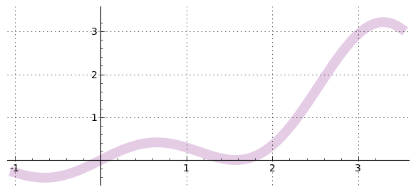
f = x*cos(x)^2 f

 $\newcommand{\Bold}[1]{\mathbf{#1}}x \cos\left(x\right)^{2}$

plot(f)

p = plot(f, xmin=-1, xmax=3.5, ymin=-0.5, ymax=3.5, aspect_ratio=.5, gridlines=True, color='purple', thickness=10, alpha=0.2, figsize=6) p

p.save('plot.pdf')

plot.pdf

plotf = plot(f, (x,-1,3.5), color='purple', thickness=3) origin = point((0,0), color='orange', alpha=.7, size=150) label = 'MacLaurin polynomial of $%s$ of degree'%latex(f) @interact def foo(j=slider(0, 20, 1, default=3, label=label)): Tjf = f.taylor(x, 0, j) plotTjf = plot(Tjf, (x,-1,3.5), color='green', thickness=1.5, fill=f) html('$%s$'%latex(Tjf)) show(plotf + plotTjf + origin, ymin=-0.5, ymax=3.5, figsize=[7,3])

MacLaurin polynomial of

xcos(x)2 $x \cos\left(x\right)^{2}$ of degree

3

Click to the left again to hide and once more to show the dynamic interactive window

frames = [] for j in range(-1, 21, 2): Tjf = f.taylor(x, 0, j) plotTjf = plot(Tjf, (x,-1,3.5), color='green', thickness=1.5, fill=f) t = text('$%s$'%latex(Tjf), (3,-0.8), color='black', horizontal_alignment='right') frames.append(t + plotf + plotTjf + origin) a = animate(frames, ymin=-0.5, ymax=3.5, figsize=[7,3]) a.show(delay=40)

var('x, y, z') f = x^2 + y^2 + z^2 + cos(4*x) + cos(4*y) + cos(4*z) c = 0.2 implicit_plot3d(f==c, (x, -1.2, 1.2), (y, -1.2, 1.2), (z, -1.2, 1.2))

Sleeping...
If no image appears re-execute the cell. 3-D viewer has been updated.

implicit_plot3d(f==c, (x, -1.2, 1.2), (y, -1.2, 1.2), (z, -1.2, 1.2), opacity=2/3) + dodecahedron((0,0,0), 1/2, color="purple", opacity=2/3)

solve(x^3 + 6*x == 20, x)

 $\newcommand{\Bold}[1]{\mathbf{#1}}\left[x = \left(-3 i - 1\right), x = \left(3 i - 1\right), x = 2\right]$

solve(x^4 + 6*x == 20, x)[0]

 $\newcommand{\Bold}[1]{\mathbf{#1}}x = -\frac{1}{2} \, \sqrt{\frac{3 \, {\left(\frac{2}{9} \, \sqrt{3} \sqrt{130187} + 18\right)}^{\left(\frac{2}{3}\right)} - 80}{{\left(\frac{2}{9} \, \sqrt{3} \sqrt{130187} + 18\right)}^{\frac{1}{3}}}} \sqrt{\frac{1}{3}} - \frac{1}{2} \, \sqrt{-{\left(\frac{2}{9} \, \sqrt{3} \sqrt{130187} + 18\right)}^{\left(\frac{1}{3}\right)} + \frac{36 \, \sqrt{\frac{1}{3}}}{\sqrt{\frac{3 \, {\left(\frac{2}{9} \, \sqrt{3} \sqrt{130187} + 18\right)}^{\left(\frac{2}{3}\right)} - 80}{{\left(\frac{2}{9} \, \sqrt{3} \sqrt{130187} + 18\right)}^{\frac{1}{3}}}}} + \frac{80}{3 \, {\left(\frac{2}{9} \, \sqrt{3} \sqrt{130187} + 18\right)}^{\left(\frac{1}{3}\right)}}}$

solve(x^5 + 6*x == 20, x)

 $\newcommand{\Bold}[1]{\mathbf{#1}}\left[0 = x^{5} + 6 \, x - 20\right]$

find_root(x^5 + 6*x == 20, 0, 1)

Traceback (click to the left of this block for traceback)
...
RuntimeError: f appears to have no zero on the interval

Traceback (most recent call last):
  File "<stdin>", line 1, in <module>
  File "_sage_input_7.py", line 10, in <module>
    exec compile(u'open("___code___.py","w").write("# -*- coding: utf-8 -*-\\n" + _support_.preparse_worksheet_cell(base64.b64decode("ZmluZF9yb290KHheNSArIDYqeCA9PSAyMCwgMCwgMSk="),globals())+"\\n"); execfile(os.path.abspath("___code___.py"))
  File "", line 1, in <module>
    
  File "/private/var/folders/ml/70rrwtg15qzbrggwjj6s2z800000gn/T/tmpqm_dZy/___code___.py", line 3, in <module>
    exec compile(u'find_root(x**_sage_const_5  + _sage_const_6 *x == _sage_const_20 , _sage_const_0 , _sage_const_1 )
  File "", line 1, in <module>
    
  File "/Applications/Sage.app/Contents/Resources/sage/local/lib/python2.7/site-packages/sage/numerical/optimize.py", line 76, in find_root
    return f.find_root(a=a,b=b,xtol=xtol,rtol=rtol,maxiter=maxiter,full_output=full_output)
  File "expression.pyx", line 8806, in sage.symbolic.expression.Expression.find_root (sage/symbolic/expression.cpp:35998)
  File "/Applications/Sage.app/Contents/Resources/sage/local/lib/python2.7/site-packages/sage/numerical/optimize.py", line 108, in find_root
    raise RuntimeError("f appears to have no zero on the interval")
RuntimeError: f appears to have no zero on the interval

find_root(x^5 + 6*x == 20, 0, 2)

 $\newcommand{\Bold}[1]{\mathbf{#1}}1.59778267898$

var('x, y, z') solve([x + 3*y - 2*z == 5, 3*x + 5*y + 6*z == 7], x, y, z)

 $\newcommand{\Bold}[1]{\mathbf{#1}}\left[\left[x = -7 \, r_{1} - 1, y = 3 \, r_{1} + 2, z = r_{1}\right]\right]$

A = matrix([[1, 3, -2], [3, 5, 6]]) v = vector([5, 7]) A.solve_right(v)

 $\newcommand{\Bold}[1]{\mathbf{#1}}\left(-1,\,2,\,0\right)$

A.right_kernel()

 $\newcommand{\Bold}[1]{\mathbf{#1}}\mathrm{RowSpan}_{\Bold{Z}}\left(\begin{array}{rrr} 7 & -3 & -1 \end{array}\right)$

Av = A.augment(v) Av.echelon_form()

 $\newcommand{\Bold}[1]{\mathbf{#1}}\left(\begin{array}{rrrr} 1 & 3 & -2 & 5 \\ 0 & 4 & -12 & 8 \end{array}\right)$

type(Av)

 $\newcommand{\Bold}[1]{\mathbf{#1}}\verb|<type|\phantom{\verb!x!}\verb|'sage.matrix.matrix_integer_dense.Matrix_integer_dense'>|$

Av = Av.change_ring(QQ) type(Av); Av.echelon_form()

 $\newcommand{\Bold}[1]{\mathbf{#1}}\verb|<type|\phantom{\verb!x!}\verb|'sage.matrix.matrix_rational_dense.Matrix_rational_dense'>|$ 
 $\newcommand{\Bold}[1]{\mathbf{#1}}\left(\begin{array}{rrrr} 1 & 0 & 7 & -1 \\ 0 & 1 & -3 & 2 \end{array}\right)$

S4 = SymmetricGroup(4)

S4

Symmetric group of order 4! as a permutation group

Symmetric group of order 4! as a permutation group

show(S4)

 $⟨ (1, 2, 3, 4), (1, 2) ⟩$  $\newcommand{\Bold}[1]{\mathbf{#1}}\langle (1,2,3,4), (1,2) \rangle$

S4.conjugacy_classes_representatives()

[(), (1,2), (1,2)(3,4), (1,2,3), (1,2,3,4)]

[(), (1,2), (1,2)(3,4), (1,2,3), (1,2,3,4)]

len(S4.conjugacy_classes_representatives()), len(S4.subgroups()), len(S4.conjugacy_classes_subgroups()), len(S4.normal_subgroups())

(5, 30, 11, 4)

(5, 30, 11, 4)

u = S4( (1,2,3,4) ) v = S4( (2,4) ) w = S4( ((1,2),(3,4)) )

u.order(), u*v, w==u^-1*v

(4, (1,4)(2,3), True)

(4, (1,4)(2,3), True)

G = S4.subgroup([u, v])

G.order(), G.is_abelian(), G.center().order(), G.is_isomorphic(DihedralGroup(4))

(8, False, 2, True)

(8, False, 2, True)

(1,4) in G, (1,3) in G

(False, True)

(False, True)

G.cayley_graph(generators=[u, v]).show(color_by_label=True)

G.cayley_graph(generators=[v, w]).show(color_by_label=True)

T = G.cayley_table() T

*  a b c d e f g h
 +----------------
a| a b c d e f g h
b| b a d c f e h g
c| c g a e d h b f
d| d h b f c g a e
e| e f g h a b c d
f| f e h g b a d c
g| g c e a h d f b
h| h d f b g c e a

*  a b c d e f g h
 +----------------
a| a b c d e f g h
b| b a d c f e h g
c| c g a e d h b f
d| d h b f c g a e
e| e f g h a b c d
f| f e h g b a d c
g| g c e a h d f b
h| h d f b g c e a

T.translation()

{'a': (), 'c': (1,2)(3,4), 'b': (2,4), 'e': (1,3), 'd': (1,2,3,4), 'g':
(1,4,3,2), 'f': (1,3)(2,4), 'h': (1,4)(2,3)}

{'a': (), 'c': (1,2)(3,4), 'b': (2,4), 'e': (1,3), 'd': (1,2,3,4), 'g': (1,4,3,2), 'f': (1,3)(2,4), 'h': (1,4)(2,3)}

from sage.matrix.operation_table import OperationTable def commutator(h, g): return h*g*h^-1*g^-1 OperationTable(G, commutator)

.  a b c d e f g h
 +----------------
a| a a a a a a a a
b| a a f f a a f f
c| a f a f f a f a
d| a f f a f a a f
e| a a f f a a f f
f| a a a a a a a a
g| a f f a f a a f
h| a f a f f a f a

.  a b c d e f g h
 +----------------
a| a a a a a a a a
b| a a f f a a f f
c| a f a f f a f a
d| a f f a f a a f
e| a a f f a a f f
f| a a a a a a a a
g| a f f a f a a f
h| a f a f f a f a

R.<a,b,c,d,e> = PolynomialRing(QQ) I = R.ideal([a*c, b*d, a*e, d*e]) R; I

Multivariate Polynomial Ring in a, b, c, d, e over Rational Field
Ideal (a*c, b*d, a*e, d*e) of Multivariate Polynomial Ring in a, b, c,
d, e over Rational Field

Multivariate Polynomial Ring in a, b, c, d, e over Rational Field
Ideal (a*c, b*d, a*e, d*e) of Multivariate Polynomial Ring in a, b, c, d, e over Rational Field

I.syzygy_module()

[  -e    0    c    0]
[   0   -e    0    b]
[   0    0   -d    a]
[-b*d  a*c    0    0]

[  -e    0    c    0]
[   0   -e    0    b]
[   0    0   -d    a]
[-b*d  a*c    0    0]

singular.mres(I, 0)

[1]:
   _[1]=d*e
   _[2]=a*e
   _[3]=b*d
   _[4]=a*c
[2]:
   _[1]=c*gen(2)-e*gen(4)
   _[2]=b*gen(1)-e*gen(3)
   _[3]=a*gen(1)-d*gen(2)
   _[4]=a*c*gen(3)-b*d*gen(4)
[3]:
   _[1]=a*c*gen(2)-b*c*gen(3)-b*d*gen(1)+e*gen(4)
[4]:
   _[1]=0
[5]:
   _[1]=gen(1)

[1]:
   _[1]=d*e
   _[2]=a*e
   _[3]=b*d
   _[4]=a*c
[2]:
   _[1]=c*gen(2)-e*gen(4)
   _[2]=b*gen(1)-e*gen(3)
   _[3]=a*gen(1)-d*gen(2)
   _[4]=a*c*gen(3)-b*d*gen(4)
[3]:
   _[1]=a*c*gen(2)-b*c*gen(3)-b*d*gen(1)+e*gen(4)
[4]:
   _[1]=0
[5]:
   _[1]=gen(1)

An Introduction to Sage

Marco Varisco

Algebra/Topology Seminar, February 7, 2013

Sage as a (smart) calculator

A simple algorithm

Some calculus and pretty pictures

Click to the left again to hide and once more to show the dynamic interactive window

Solving equations

Playing with finite groups

Minimal free resolutions of monomial ideals

And don’t forget the SageTeX example! $\infty$

An Introduction to Sage

Marco Varisco

Algebra/Topology Seminar, February 7, 2013

Sage as a (smart) calculator

A simple algorithm

Some calculus and pretty pictures

Click to the left again to hide and once more to show the dynamic interactive window

Solving equations

Playing with finite groups

Minimal free resolutions of monomial ideals

And don’t forget the SageTeX example! ∞\infty

And don’t forget the SageTeX example! $\infty$