CHAPTER 1: Management Accounting Defined, Described, and Compared to Financial Accounting

MANAGEMENT ACCOUNTING CONCEPTS AND TECHNIQUES

By Dennis Caplan, University at Albany (State University of New York)

�

CHAPTER 5: Cost-Volume-Profit

Chapter Contents:

- The Basic Profit Equation

- Assumptions in CVP analysis

- Target costing

- Leverage

- Constrained resources

- Examples

- Exercises and problems

The Basic Profit Equation:

Cost-Volume-Profit analysis (CVP) relates the firm�s cost structure to sales volume and profitability. A formula that facilitates CVP analysis can be easily derived as follows:

�� Profit �� = �� Sales � Expenses

�� Profit�� =�� Sales � (Variable Costs + Fixed Costs)

�� Profit + Fixed Costs � = �� Sales � Variable Costs

�� Profit + Fixed Costs � =�� Units Sold x (Unit Sales Price � Unit Variable Cost)

This formula is henceforth called the Basic Profit Equation and is abbreviated:

�� P + FC = Q x (SP � VC)

Contribution margin is defined as �

Sales � Variable Costs

The unit contribution margin is defined as

�� Unit Sales Price � Unit Variable Cost

Typically, the Basic Profit Equation is used to solve one equation in one unknown, where the unknown can be any of the elements of the equation. For example, given an understanding of the firm�s cost structure and an estimate of sales volume for the coming period, the equation predicts profits for the period. As another example, given the firm�s cost structure, the equation indicates the required sales volume Q to achieve a targeted level of profits P. If targeted profits are zero, the equation simplifies to

�� Q = FC � Unit Contribution Margin�

In this case, Q indicates the required sales volume to break even, and the exercise is called breakeven analysis.�

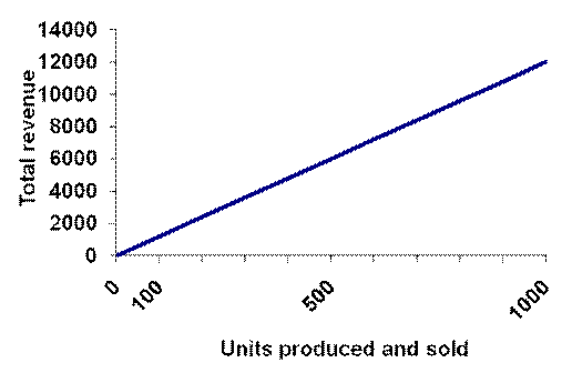
CPV analysis can be depicted graphically. The graph below shows total revenue (SP x Q) as a function of sales volume (Q), when the unit sales price (SP) is $12.�

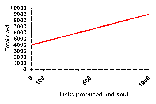
The following graph shows the total cost function when fixed costs (FC) are $4,000 and the variable cost per unit (VC) is $5.

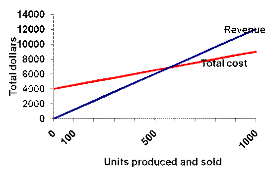
The following graph combines the revenue and cost functions depicted in the previous two graphs into a single graph.

The intersection of the revenue line and the total cost line indicates the breakeven volume, which in this example, occurs between 571 and 572 units. To the left of this point, the company incurs a loss. To the right of this point, the company generates profits. The amount of profit or loss can be measured as the vertical distance between the revenue line and the total cost line.

Assumptions in CVP Analysis:

The Basic Profit Equation relies on a number of simplifying assumptions.

1. Only one product is sold. However, multiple products can be accommodated by using an average sales mix and restating Q, SP and VC in terms of a representative bundle of products. For example, a hot dog vendor might calculate that the �average� customer buys two hot dogs, one bag of chips, and two-thirds of a beverage. Q is the number of customers, and SP and VC refer to the sales price and variable cost for this �average� customer order.

�

2. If the equation is applied to a manufacturer, beginning inventory is assumed equal to zero, and production is assumed equal to sales. Relaxing these assumptions requires additional structure on the equation, including specifying an inventory flow assumption (e.g., FIFO or LIFO) and the extent to which the matching principle is honored for manufacturing costs.

3. The analysis is confined to the relevant range. In other words, fixed costs remain unchanged in total, and variable costs remain unchanged per unit, over the range of Q under consideration.

Target Costing:

A relatively recent innovation in product planning and design is called target costing. In the context of the Basic Profit Equation, target costing sets a goal for profits, and solves for the unit variable cost required to achieve those profits. The design and manufacturing engineers are then assigned the task of building the product for a unit cost not to exceed the target. This approach differs from a more traditional product design approach, in which design engineers (possibly with input from merchandisers) design innovative products, manufacturing engineers then determine how to make the products, cost accountants then determine the manufacturing costs, and finally, merchandisers and sales personnel set sales prices. Hence, setting the sales price comes last in the traditional approach, but it comes first in target costing.

Target costing is appropriate when SP and Q are predictable, but are not choice variables, such as might occur in well-established competitive markets. In such a setting, merchandisers might know the price that they want to charge for the product, and can probably estimate the sales volume that will be achieved at that price. Target costing has been used successfully by a number of companies including Toyota, which redesigned the Camry around the turn of the century as part of a target costing strategy.��

Constrained Resources:

Contribution margin analysis plays an important role when a multi-product organization has a binding resource constraint. The resource constraint can take many forms, such as production throughput on a critical machine, freezer space, or skilled labor hours in a particular function. In the presence of a resource constraint, the optimal production decision is to maximize the contribution margin per unit of the constraint.

For example, assume that a company makes small widgets and large widgets. Small widgets incur $5 in variable manufacturing and non-manufacturing costs, and sell for $10. Large widgets incur $11 in variable manufacturing and non-manufacturing costs, and sell for $15. If production throughput is constrained by the capacity of a particular machine, and both small and large widgets require one hour of processing time on that machine, then the company should make only small widgets, because small widgets provide a contribution margin of $5 per unit, whereas large widgets provide a contribution margin of $4 per unit. On the other hand, if each small widget requires two hours of processing time on the machine, and large widgets require only one hour, then the company should make only large widgets, calculated as follows:

Small widgets: contribution margin per machine hour = ($10 - $5) � 2 = $2.50 per hour

Large widgets: contribution margin per machine hour = ($15 - $11) � 1 = $4.00 per hour

The company maximizes profits by making large widgets, even though large widgets have a lower contribution margin per unit than small widgets, because large widgets require less machine time and hence, are more efficient with respect to the limited resource. In other words, the large widgets generate a higher contribution margin per hour on the machine that constitutes the capacity constraint of the factory.

Leverage:

There is often a trade-off between fixed cost inputs and variable cost inputs. For example, in the manufacturing sector, a company can build its own factory (thereby operating with relatively high fixed costs but relatively low variable costs) or outsource production (operating with relatively low fixed costs but relatively high variable costs). A merchandising company can pay its sales force a flat salary (relatively higher fixed costs) or rely to some extent on sales commissions (relatively higher variable costs). A restaurant can purchase the equipment to launder table cloths and towels, or it can hire a laundry service.

A company that has relatively high fixed costs is more highly leveraged than a company with relatively high variable costs. Higher fixed costs result in greater downside risk: as Q falls below the breakeven point, the company loses money more quickly than a company with less leverage. On the other hand, the company�s lower variable costs result in a higher unit contribution margin, which means that as Q rises above the breakeven point, the more highly-leveraged company is more profitable.��

There is an ongoing trend for companies to outsource support functions and other �non-core� activities to third party suppliers and providers. Usually, outsourcing reduces the leverage of the company by eliminating the fixed costs associated with conducting those activities inside the firm. When the activities are outsourced, the contractual payments to the outsource providers usually contain a large variable cost component and a relatively small or no fixed cost component.��

Examples:

Breakeven: Steve Poplack owns a service station in Walnut Creek. Steve is considering leasing a machine that will allow him to offer customers the mandatory California emissions test. Every car in the state must be tested every two years. The machine costs $6,000 per month to lease. The variable cost per test (i.e., per car inspected) is $10. The amount that Steve can charge each customer is set by state law, and is currently $40.

How many inspections would Steve have to perform monthly to break even from this part of his business?

�

Q = FC � Unit Contribution Margin�

Q = $6,000 � ($40 - $10) = 200 inspections

Targeted profits, solving for volume: Refer to the information in the previous question. How many inspections would Steve have to perform monthly to generate a profit of $3,000 from this part of his business?�

P + FC = Q x (SP � VC)

$3,000 + $6,000 = Q x ($40 - $10)

Q = 300 inspections

Targeted profits, solving for sales price: Alice Waters (age 9) runs a lemonade stand in the summer in Palo Alto, California. Her daily fixed costs are $20. Her variable costs are $2 per glass of ice-cold, refreshing, lemonade. Alice sells an average of 100 glasses per day. What price would Alice have to charge per glass, in order to generate profits of $200 per day?

P + FC = Q x (SP � VC)

$200 + $20 = 100 x (SP - $2)

SP = $4.20 per glass

Contribution margin: Refer to the previous question. What price would Alice have to charge per glass, in order to generate a total contribution margin of $200 per day?

Total CM = Q x (SP � VC)

$200 = 100 x (SP - $2.00)

SP = $4.00 per glass

Target costing: Refer to the information about Alice, but now assume that Alice wants to charge $3 per glass of lemonade, and at this price, Alice can sell 110 glasses of lemonade daily. Applying target costing, what would the variable cost per glass have to be, in order to generate profits of $200 per day?

P + FC = Q x (SP � VC)

$200 + $20 = 110 x ($3 � VC)

VC = $1

Go to the End-of-Chapter Exercises and Problems

Go to the Next Chapter

Return to the Table of Contents

For a printer-friendly version, contact Dennis Caplan at [email protected]